Friday, October 12, 2012

Kimball Conference Lessons Learned

I recently had the distinct privilege of attending Ralph Kimball's Dimensional Modeling In Depth class, as described in this post. Learning directly from icons such as Ralph Kimball and Margy Ross has been a huge blessing and a very enjoyable experience.  One of the most eye-opening (and valuable) experiences has involved tweaking my understanding regarding concepts that I thought I understood...but found that I didn't. Some of these misunderstandings have even come out in this blog, so I'll use this post to correct some of those...

1.) Junk Dimensions - The examples of junk dimensions that I have provided included the word "junk" in the name.  Margy Ross suggests not naming it as such, which makes a lot of sense.  Encountering a table with junk in the name may cause some confusion (perhaps even concern) for an analyst who is not well-versed in dimensional modeling.

2.) Snowflake Schema - The terms portion of my website provides the following definition for a snowflake schema

Occasionally there are reasons to join one dimension table to another dimension table. A schema in which this occurs is referred to as a snowflake schema. The ERD, in this case, will show this “second layer” of dimension tables as being similar in appearance to a snowflake.

This dimensional modeling class proved to me that this definition is a bit misleading.  Joining one dimension table to another, such as the one on the terms portion of my website, is referred to as an outrigger.  A snowflake schema involves an attempt to completely denormalize a dimension.

3.) Type 3 Slowly Changing Dimension - In this post, I described Type 3 slowly changing dimensions as being a hybrid between type 1 and type 2.  In reality, this hybrid is actually referred to as a type 6 (I need to update the other post).  So, what is a type 3 slowly changing dimension?  I'll save that explanation for a future post; however, the type 3 is not the hybrid that I thought it was.

One of the advantages of attending a course like this is that you get to bounce your knowledge against some of the most brilliant minds in the industry.  In some cases they help to affirm what you already know.  In other cases they correct what you already "know"...which turns you into a stronger asset for your organization and for the industry. 

For more information on data warehousing concepts visit www.brianciampa.com.  For data that can be used to practice modeling and/or ETL, click on Career in Data Warehousing and then click Grow.  Also, if you need a fresh approach to marketing your data warehousing skillset, consider The Data Warehouse Portfolio.

Saturday, October 6, 2012

Kimball University

Just as a young quarterback would be thrilled to meet Peyton Manning or a young cook would jump at the chance to meet Paula Dean, I enjoyed that experience this week in the context of my vocation.  I sat at the feet of Margy Ross and Ralph Kimball.  When you mention these names amongst non-data warehousing professionals, you are often met with confused looks.  However, those in the data warehousing arena know these individuals as some of the most brilliant minds when it comes to modeling data. 

Margy Ross spent the first two days polishing our skills on some of the more basic pieces of dimensional modeling.  She is a very professional yet light-hearted lady with a true talent for teaching these concepts.  I was blessed to learn that I had a few things wrong regarding some concepts that I thought I understand.  Some of those have even come out in this blog; the corrections for which I'll save for a future post.

Ralph Kimball spent days three and four going over some advanced concepts with regards to dimensional modeling (and a bit of ETL).  He is just as light-hearted, having the ability to explain very complex data warehousing concepts with humor inserted where appropriate.  I spent a fair portion of the class laughing, and I still smile as I remember their humor.  This was not a dry class, as some would expect (for those who enjoy data warehousing, that is).  Both Margy and Ralph are brilliant minds who have the humility to (1) impart some of their knowledge to serious data warehousing students in an interesting way and (2) answer concise questions that apply to your specific organization in a one-on-one setting (assuming you can catch them after class).  Here were some of my personal highlights...

1.) Ralph signed my copy of The Data Warehouse Toolkit by writing "Brian, keep to the grain.  Ralph Kimball".

2.) I've had a design conundrum at work regarding a many-to-many problem related to this post.  I asked him about it after class and he affirmed my suggested solution.

3.) Ralph began his first class on day three by explaining the way in which a data warehouse developer will begin asking a user what needs to exist in that user's data warehouse (which does not involve asking the question in that exact way).  As a part of that conversation, Ralph made an example out of yours truly, as though I were a successful account manager looking to implement a data warehouse. Of course he was painting a fictitious scenario to make his point but it was still a cool moment.

I would highly recommend the Dimensionsal Modeling In Depth course to anybody interested in the data warehousing arena.  I'm not affiliated with the Kimball Group in any way (other than being a fan) so I will not profit by anybody taking the course.  I recommend it because it is simply that good.

Image courtesy of smokedsalmon / FreeDigitalPhotos.net

Friday, September 28, 2012

Data Extraction Techniques

One of the challenges of writing ETL involves deciding which records to pull from the source system.  If a salary star schema is built to contain payroll data, then the ETL job will refresh on a recurring basis to add new data to that star.  If some data related to salary dollars already exists in the star and some new data makes it into the source system, how can the ETL job know to load the new data into the star and avoid reloading the records that were previously loaded (since they already exist in the data warehouse)?  There is no one way of doing this, but consider these options...

1.) Use the source system's datetime stamps - An ETL developer should consider himself very blessed if his source system contains an insert and update datetime stamp for each record in the system.  If this is the case, then he can simply store the date and time of the most recent successful extract and then pull everything that has been inserted or updated since then.  It will be important for the ETL developer to understand how those audit columns are populated in each table to make sure that necessary data will not be left out and unnecessary data will not be included due to odd occurances (i.e., a source system table is reloaded for some reason and records that pertain to data that was initially added three years ago have yesterday's timestamp, etc.).

2.) Compare to the prior extract - In his book The Data Warehouse ETL Toolkit : Practical Techniques for Extracting, Cleaning, Conforming, and Delivering Data, Ralph Kimball suggests always saving the prior extract in the staging area.  A new extract can be compared to this prior extract and the differences will be uploaded.  Finally the new extract will overwrite the prior extract and be used as the baseline for the next update.

3.) Always pull as of a certain date - In this approach, the salary dollars may always be extracted for the current calendar year (for example).  So, as the year goes on each extraction will be slightly larger than the last.  In April, all salary dollars that date back to January will be extracted from the source.  In May, all salary dollars that date back to January will be extracted from the source as well.  When using this option in conjunction with loading a fact table, the ETL developer will need to delete all of the applicable year's records from the fact table and then load the extract.  Although several records will be deleted and simply reloaded (with no change), this is one way of grabbing what is needed from the source when a simpler solution is not possible.  However, any updates made to the data that pertain to a different year will be missed.  This will need to be taken into consideration.  When using this option in conjunction with loading a dimension table, the ETL developer will need to compare to the dimension table to see if any of the dimensions have changed and only load or update the changes.  Deleting records from the dimension table and reloading is not a good strategy since the fact table has foreign keys that reference the dimension table.

4.) Refresh the fact table - In this case all of the data from the source system will always be extracted and the fact table will be truncated and reloaded each time.  This will only be an acceptable solution if the fact table can be loaded in a timely fashion.  Also, this will only be acceptable with a fact table most of the time.  Even if an ETL developer plans to refresh an entire star (fact and dimension tables) she must consider the possibility that some of these dimensions are conformed dimensions, meaning that other fact tables reference them.

There are obviously more options than these four.  With whatever option you choose, it is important to build the job so that it can be run multiple times with no negative impact.  In other words, running the job twice should not result in duplicate records showing up.  Even though the initial extract may place more records than are needed into the staging area, the job should be "smart enough" to know exactly what to load into the data warehouse and what to exclude.

For more information on data warehousing techniques as well as data with which you can practice writing your own ETL, visit www.brianciampa.com/careerindatawarehousing/grow.html.  Also, if you need a fresh approach to marketing your skillset, consider The Data Warehouse Portfolio.

Image courtesy of digitalart / FreeDigitalPhotos.net

Friday, September 21, 2012

To Constrain or Not Constrain

One of the advantages of using a relational database is that you can mandate that certain relationships MUST exist within your data.  If somebody tries to enter data into the database that does not relate to other data correctly, the database can be configured to reject that "bad data" until it is corrected.  Since many data warehouses reside in relational databases, using this feature is an option for the data warehousing team as well. 

Consider this example...suppose that a star contains a DIM_PRODUCT table that contains the products that are used by that business process.  If the Men's Raincoat product has a KEY_PRODUCT value of 27 (surrogate key) then the records in the corresponding fact tables that pertain to this product will have a KEY_PRODUCT value of 27 (foreign key).  That's a lesson from Database 101.  If somebody removes the Men's Raincoat product from the DIM_PRODUCT table while records that point to it exist in the fact table, then those fact table records will point to nothing...and become meaningless.

The advantage of enforcing this constraint within the database itself is that if somebody tries to remove the Men's Raincoat product from the DIM_PRODUCT table the database will not allow it until the "child records" from the fact table have been deleted or repointed.  Using this feature sounds like a no-brainer (and it may be) but a data warehouse provides an additional twist to this kind of decision since so much data is being inserted.

Option 1: Enforce Constraints - This will ensure that the relationship between the fact and dimension tables are always valid from a technical perspective.  However, each time that the data is loaded via the ETL job, the fact table must look to make sure that a parent record exists in the dimension.  If (and only if) it exists, it will load that record into the fact.  Doing that for each and every record will ensure good data intregity but it can also slow a job down.

Option 2: Do Not Enforce Constraints - This will probably result in a faster and more efficient ETL job.  However, the possiblity of the fact table containing some orphan records exists.

It is up to each data warehousing team to decide which is best for their particular situation.  In some cases it is appropriate to physically enforce constraints (option 1).  In other cases, it may be appropriate to logically enforce constraints (option 2), meaning that the data warehousing team will need to periodically run SQL statements that specifically look for orphaned records. 

If you are looking for more information on data warehousing and/or data that can be used to practice ETL and architecture skills, visit www.brianciampa.com and click on Career in Data Warehousing.  Also, if you are looking for a fresh way to market your data warehousing skills, consider The Data Warehouse Portfolio.

Image: FreeDigitalPhotos.net

Friday, September 14, 2012

Bridge Tables

Each of the examples that we've used thus far in this blog have involved situations in which each fact row was associated with only on dimension row, per dimension table.  In other words there has always been a many-to-one relationship between the fact table and its associated dimensions.  In the real world, this relationship will not always be the case. 

Suppose that a fact table contains employee salary data and each employee can be associated with multiple departments at once.  Conceptually, the design would be something like this...


One possible way of resolving this is to use what some people call a bridge table.  This is essentially a crosswalk between the fact and dimension designed to resolve the many-to-many problem.  The design for such a table is below.


The EMPLOYEE_DEPT_BRIDGE table will not contain any data that will be seen in query results.  It will only be used as a link between the FACT_SALARY and the DIM_DEPARTMENT tables.  However, there is a rule that must be well understood by any and all analysts that select from this table: You must always group by the department in your query results if your select statement joins to the DIM_DEPARTMENT table (via the bridge, of course) in any way.  For example, suppose that John Smith (KEY_EMPLOYEE value is 123) has $1,000 in wages and is associated with both accounting and human resources (part time in each, perhaps).  Consider this SQL statement...

select a.key_employee_name,
sum(a.wage_amount)
from fact_salary a,
employee_dept_bridge b,
dim_department c
where a.key_employee = b.key_employee
and b.key_department = c.key_department
and a.key_employee = 123
group by a.key_employee_name

Because the EMPLOYEE_DEPT_BRIDGE table will contain two rows for John Smith (one for accounting and one for human resources), these results will show a salary of $2,000 which will appear incorrect to the user. 

KEY_EMPLOYEESUM(A.WAGE_AMT)
1232,000


Now, consider this SQL statement...

select a.key_employee_name,
department_name,
sum(a.wage_amount)
from fact_salary a,
employee_dept_bridge b,
dim_department c
where a.key_employee = b.key_employee
and b.key_department = c.key_department
and a.key_employee = 123
group by a.key_employee_name,
department_name

The results will show his $1,000 salary associated with each department.  This will appear to be more correct to the user, assuming they understand that he is associated with both departments. 

KEY_EMPLOYEEDEPARTMENT_NAMESUM(A.WAGE_AMT)
123ACCOUNTING1,000
123HUMAN RESOURCES1,000


In this case, educating your analysts and report writers to use this table correctly is a key component to the success of this design.

Friday, September 7, 2012

ETL - Practice Loading A Fact - Solution

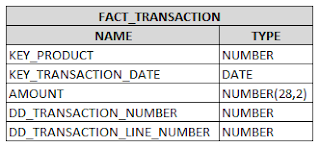
In a prior post we looked at the process by which a fact table is loaded.  I need to apologize, since the ERD of the FACT_TRANSACTION table that I posted in that prior post was incorrect.  It has since been updated.  The four things that an ETL job needs to accomplish are...

1.) Select all necessary data from the source
 a. Measures
 b. Natural Keys of the dimension objects
 c. Degenerate Dimension objects
2.) Transform the data as needed
 a. Aggregate measures and group by the appropriate objects
 b. Add foreign keys to dimension tables
3.) Delete any existing rows from the fact table that will be replaced by the new data
4.) Load the fact table

Consider this PL/SQL procedure as a procedure that will accomplish these things.

Extract

The STAGE_TRANSACTION_DATA table pulls all of the necessary elements from the source system into the staging area.  I am treating one schema as both the staging area and the presentation area.  This is probably unrealistic in a production environment but it keeps things simple for these purposes.

Transform

1.) The STAGE_TRANS_DATA_PROD_KEY table is used to grab the KEY_PRODUCT from the DIM_PRODUCT dimension.  Notice that this is done by joining the product's natural key, which is the PRODUCT_NO (product number), to the DIM_PRODUCT table.  An outerjoin is used so that if a record comes into the staging area for a product that does not exist in the DIM_PRODUCT table, that record will not be excluded from the fact table.  It will exist with a value of -1 and will need to be addressed after the ETL has run.

2.) The STAGE_TRANS_DATA_DATE_KEY table is used to transform the TRANSACTION_DATE into a key that will join to a date dimension.  I created the date dimension on my own, so I'll let you try and tackle that one.  Those dimensions typically have no source and are created as needed by the ETL developer.  Again, an outer join is used so that if a date does not exist in that dimension a value of -1 is placed into the fact table.

Load

1.) This fact table, because it is so small, is truncated and then repopulated each time that the ETL runs.  Date logic can be written so that only a certain time period will be refreshed with each run, but for simplicity's sake I did it this way.

2.) Finally, the data is loaded into the FACT_TRANSACTION table.

Prior posts have talked about turning data into valuable data.  This post shows you how to accomplish that in a hands-on way.

Remember to take a look at www.brianciampa.com (specifically, click on Career In Data Warehousing and then Grow) for larger datasets that can be used for this kind of practice. 

Image: FreeDigitalPhotos.net

Wednesday, September 5, 2012

Tales of Work

I typically do not blog in the middle of the week, but this week I'll make an exception.  Kimanzi Constable is a career coach who maintains a great blog, called Tales of Work, on discovering your talents and finding work that you enjoy.  He has been gracious enough to run a guest post that I wrote on the portfolio concept.  You can check out the guest post here.

My blog is built on the premise that data warehousing and business intelligence are about helping decision makers to see the true value in their data.  Those decision makers are best helped by those who are passionate about data.  That best describes me, which is why I maintain the Valuable Data blog in hopes of helping other passionate people to hone that skill.  If you find yourself needing some help in finding your passion, consider the Tales of Work blog.

Image: Courtesy of FreeDigitalPhotos.net

Sunday, September 2, 2012

ETL - Practice Loading A Fact

We looked recently at the process used to load a dimension table.  Consider this post as a way to practice loading a fact table.  An ETL job that is designed to load a fact table will accomplish these things…
1.)    Select all necessary data from the source
a.       Measures
b.      Natural Keys of the dimension objects
c.       Degenerate Dimension objects
2.)    Transform the data as needed
a.       Aggregate measures and group by the appropriate objects
b.      Add foreign keys to dimension tables
3.)    Delete any existing rows from the fact table that will be replaced by the new data
4.)    Load the fact table

As with the dimension example, no two developers will do this the same way, which is perfectly fine.  Consider this example which is to be used in conjunction with the two tables used in the ETL – Practice Loading a Dimension post (click on the image to enlarge it)…


…and this fact table needs to be populated.

Run the following scripts in Oracle to create the source data

1.)    Product data – This is the same script from the ETL – Practice Loading a Dimension post.  If you have already run this one, you are fine.
2.)    Transaction data - This script will create and populate the TRANSACTION_HEADER and TRANSACTION_DETAIL tables above.

The TRANSACTION_DETAIL.PRODUCT_ID is a foreign key to the PRODUCT.ID field from the ETL – Practice Loading a Dimension post.  If you wish, try to write an ETL job that will populate the FACT_TRANSACTION table in PL/SQL or another language of your choosing.  We will examine a possible solution in a future post.

For more practice data and additional information on dimensional modeling visit www.brianciampa.com.  Also, if you need a fresh approach to marketing your data warehousing skillset consider The Data Warehouse Portfolio.

Saturday, August 25, 2012

Dimensional Modeling Video


Dimensional modeling is a very powerful technique in helping to enable excellent decision making.  This is a video that explains the business value that can be derived from using this technique.  For more information on dimensional modeling, including free data with which you can practice, look at the Learn, Grow, and Succeed links at http://www.brianciampa.com/careerindatawarehousing.html

Also, for those looking for a fresh way to market your skillset consider The Data Warehouse Portfolio at http://www.brianciampa.com

Friday, August 17, 2012

The Data Warehouse Portfolio

You've spent weeks in data warehousing classes, days in training sessions, hours reading books on the subject, and perhaps years warehousing data for other organizations.  However, right now you want to work for this one.  You know that you have the experience as well as the ambition.  You have a list of ideas to take to this new potential employer that you know will provide immense value. So, what's the next step?  All of that is placed onto a very professionally-looking resume and submitted.  The only problem is that everybody else has done that same thing.  You are not known as "Bob, who will add huge value to the business intelligence team," you are known as applicant 27...just another resume in the stack.

Perhaps you are on the other end of the spectrum.  You are a novice looking for your first data warehousing position with no prior experience outside of class.  You need a way to actually show that despite your lack of work experience you can do this...and do it well.

Do you need a fresh approach to marketing your skillset in hopes of standing out in the crowd?  It is interesting that those in the event industry are expected to provide samples of their work for potential clients.  Cake decorators, wedding photographers, and other similar vendors would probably be passed over if they only provided a resume that explained what they had done before or what their education claims that they are capable of doing.

What if you placed a sample of your data warehousing skillset onto the web specifically for a potential employer to browse?  In other words, you would have a resume to provide the details of your experience and education and a portfolio to provide an example of what you can actually do.  The Data Warehouse Portfolio is a book that suggests a way to accomplish this.  More information is available at www.brianciampa.com.  You may also want to revisit this prior blog post for a bit more information as well.

Your job is to turn data into valuable data.  However, showing the value in yourself is the first step in getting that job.

Friday, August 10, 2012

ETL - Practice Loading a Dimension - Solution

In the previous post we looked at the process used to write a basic ETL job to populate a dimension table.  As discussed previously, while no two developers will write one exactly the same way, an ETL job that populates a dimension table will need to accomplish the following...

1.) Extract all of the dimension attributes from the source.
2.) Transform the data according to the requirements (i.e., concatenate first name and last name to create a full name column, etc.)
3.) Identify those records that are new to the table as opposed to those records that already exist in the table and may need to be updated due to updates in the source system
4.) Generate new surrogate key values and add them to the new records
5.) Load the records into the dimension table

Consider this example of an Oracle PL/SQL procedure that will populate the DIM_PRODUCT table.  Before running the procedure keep these things in mind...

1.) I made an error in the SQL file from the previous post, so you may want to re-download that and run it again.  The DIM_PRODUCT.PRODUCT_EFFECTIVE_FLAG should be named DIM_PRODUCT.PRODUCT_ACTIVE_FLAG. 
2.) This job depends on an Oracle sequence to create the surrogate keys.  Before running the job, run this statement in your Oracle environment...

CREATE SEQUENCE
SEQ_DIM_PRODUCT 
MINVALUE 0
INCREMENT BY 1
START WITH 1;

3.) I'll encourage you not to get too lost in the Oracle syntax.  The point is to examine the logical flow of an ETL job.  If you have a better way of structuring the Oracle code (or want to use something other than Oracle), then by all means do that.

Run the procedure (after you have created the sample data provided in the previous post, of course) to populate the DIM_PRODUCT dimension.  Notice what is happening...

1.) Extract all of the dimension attributes from the source - Everything is pulled from the source system and placed into the STAGE_PRODUCT_EXTRACT table.
2.) Transform the data according to the requirements (i.e., concatenate first name and last name to create a full name column, etc.) - The PRODUCT_ACTIVE_FLAG is derived and that data is placed into the STAGE_PRODUCT_TRANSFORM table.
3.) Identify those records that are new to the table as opposed to those records that already exist in the table and may need to be updated due to updates in the source system - New records are identified (via an outer join) and placed into the STAGE_PRODUCT_LOAD table. 
4.) Generate new surrogate key values and add them to the new records - Surrogate keys are created in the STAGE_PRODUCT_LOAD table using the Oracle sequence mentioned earlier.
5.) Load the records into the dimension table - Existing records are updated in the DIM_PRODUCT table and the new records from the STAGE_PRODUCT_LOAD table are loaded.

This job is designed to be run as many times as necessary.  Running one time or multiple times should still result in 25 records being placed into the DIM_PRODUCT table.  This is a simple example for a few reasons, one of which is that we are working with a very small amount of data.  A more complex ETL job may examine the source system's data and somehow determine which records are new and/or have been updated before pulling them into the staging area.

Also, more complex ETL jobs may not have five simple steps, as this one does, to accomplish the five things listed above.  It may take several steps to accomplish those five things due to the complexity of the data. 

If you wish, change some of the source data to see the updates occur or tweak the ETL job to your liking.  By running this ETL job, you have just turned ordinary data into something that is truly valuable.

Image: FreeDigitalPhotos.net

Friday, August 3, 2012

ETL - Practice Loading a Dimension

We've been looking recently at the concept of extract, transform, and load (ETL) jobs.  This post will begin to examine some of the mechanics.  When loading a dimension table the ETL job should accomplish the following things...

1.) Extract all of the dimension attributes from the source.
2.) Transform the data according to the requirements (i.e., concatenate first name and last name to create a full name column, etc.)
3.) Identify those records that are new to the table as opposed to those records that already exist in the table and may need to be updated due to updates in the source system
4.) Generate new surrogate key values and add them to the new records
5.) Load the records into the dimension table

Each ETL job that populates a dimension table will need to accomplish these five things, although no two developers will develop a job exactly the same way.  To get a feel for this type of job, consider this very simple example.  A source system contains these two tables among others (click the picture to enlarge)...


...and this dimension needs to be populated...


If you have an Oracle environment available to you, run this sql file to create the two source system tables, populate them with data, and create the DIM_PRODUCT table.  Each product, as you can see, is grouped under a single product group.  The PRODUCT_EFFECTIVE_FLAG indicates whether or not a product is currently effective (current at the time of the ETL job).  If you wish, try to write an ETL job that will populate the DIM_PRODUCT table in PL/SQL or another language of your choosing.  We will examine a possible solution in a future post.

Saturday, July 21, 2012

Extract, Transform, and Load Video


As a continuation of our discussion of ETL, consider this YouTube video, which is also available at http://www.youtube.com/brianciampa.  Designing the star or snowflake schema is a great start.  However,  the ETL populates that star, thus transforming your data into something that is truly valuable.  In a future post we will look at an example of a basic ETL job in Oracle.

Friday, July 13, 2012

Extract, Transform, and Load (ETL)

In prior posts, we’ve looked a bit at the basic structure of a star schema but we have not looked at populating a star schema.  Populating a data warehouse is accomplished using an extract, transform, and load (ETL) job.  This is a job that pulls data from the source system, transforms it into a structure appropriate for the data warehouse, and then loads that data into the data warehouse.  The concept of ETL is not unlike any other craft or trade.  Consider the following…

1.)    A math student reads and understands the math problem from the textbook (extract), uses a piece of scrap paper, if calculators are not allowed, to find the solution (transform), and places the answer onto the final answer sheet (load).
2.)    A carpenter purchases wood from a supplier (extract), uses his workshop to design, measure, sand, cut, etc. (transform), and then delivers the final product to the customer (load).
Usually, the transformation piece is accomplished inside of a separate schema in the database, called a staging area.  The data from the source system is placed into this area and then restructured so that it is appropriate for the star schema, much like the math student uses the scrap paper and the carpenter uses the workshop.  It is generally accepted that this area is for the ETL developer’s eyes only.  End users do not have access to data in the staging area, much like a customer is not involved in the carpenter’s workshop and the math student does not place his chicken scratch on the sheet with the final answer.  Once that data has been transformed, it is placed into the star schema and is ready for analysis.
It may be worth noting that some variations of ETL, such as ELT (extract, load, and transform), ETLT (extract, transform, load, and transform), and others, are used to describe methods by which jobs will populate a data warehouse using a different order than the standard extract then transform then load order.  In order to encompass all of these terms, the term data integration (or something similar) is often used to describe data warehouse population in a general sense.
For more information on data warehousing concepts, remember to visit http://www.brianciampa.com/

Friday, June 29, 2012

Big Data Defined

A typical question asked of business intelligence professionals is - what is big data?  In a previous post I provided some explanation of the big data challenge.  As I've learned more about this very interesting piece of business intelligence, I believe that a more complete explanation is available.  Consider this...

Suppose you own a day care, meaning that you are in the business of caring for children each day.  You have determined that in order for you to have a truly challenging day, three things have to occur.  First, you must have a large number of kids to care for on that given day.  How large is large?  There are no hard and fast rules...large enough that your current resources are strained at best and inadequate at worst.  Second, let's assume that you have no help, meaning that you need to know what each child is doing right now.  Not knowing what one of them was doing for an hour and then finding out later that he was painting the refrigerator is not acceptable.  Third, you have a very diverse group of kids.  This does not refer to diversity with regards to race or ethnicity but diversity with regards to personality.  Some of the kids love to play outside and some inside.  Some are into puzzles and others are into riding bicycles.  As a result, keeping the kids engaged in activities that they enjoy and in which they are gifted can be challenging. 

If two of the three challenges exist, the day is still challenging but not to the same extent.  You can know what each child is doing in a diverse group if you have a small number of them.  You can deal with a large number of kids if they are ALL sitting in the same room, doing the same thing.  It's the combination of the three problems that presents a challenge.  Now, consider this in terms of big data.  Big data is characterized as having three V's. 

1.) Volume - In order to data to be considered big data it must be large.  How large is large?  I'm not so sure that there is a hard and fast boundary between "normal" data and big data in terms of size.  However, I would assume that if managing the data for the purposes of business intelligence presents problems because of its size, then this V applies.

2.) Velocity - Part of the big data problem involves dealing with the speed at which the data comes in.  Decision makers want to know what is happening in their business and in the marketplace now, as opposed to experiencing a lag.  For example, if an announcement was just made with regards to a new line of business, what are people saying about that on Twitter now?  If there is a need to stream data in some way so that it can be analyzed in real time, then this V applies.

3.) Variety - Part of the big data problem involves dealing with various types of data.  Relational databases are good at storing structured data.  Structured data is data in which each element is placed into a fixed area (such as columns and rows in a database or an XML schema) that was created for that specific element's characteristics.  Dates belong here, integers belong there, etc.  Unstructured data, such as a tweet or the body of an email message, are more free form.  In other words, there is nothing governing the type of data that is stored in those environments.  If decision makers want to analyze various types of data (such as both structured and unstructured data) then this V applies.

While challenges may exist when experiencing only one or two of the above mentioned V's, the industry generally agrees that if all three characteristics apply to your data, then you have big data.

Also, remember to visit http://www.brianciampa.com/ for more information on data warehousing and business intelligience.

Image: FreeDigitalPhotos.net

Friday, June 22, 2012

Snowflake Schema

Going back to the piggy bank example from this blog's first post, we know that the value of a data warehouse lies with allowing a user to analyze data easily.  This is mainly achieved through denormalization.  This often differs from the value of a source system which lies with getting data into the system quickly.  This is mainly achieved through normalization.

So, if we were to run a select statement against a source system that is designed to return (among other things) an employee name as well as his department, those two things may be stored in two tables.  The employee table may simply store a foreign key to the department table, which stores the names of the departments.  The query may find 'John Smith' in the employee table and then the number 6 in the department field.  The database will have to go to the department table, look up the row with the number 6 to see that the value is 'Human Resources' and then return those two values, along with any other values that were specified in the select statement, in the query results.  Doing this for several rows and for several different kinds of values will take some time.

In a typical data warehouse design, however, all of these values may exist in the same table and be repeated.  This way, the query can go to one table and find 'John Smith' and 'Human Resources' without having to translate a foreign key.  This keeps things quick.

However, there are some instances in which some normalization is appropriate in a star schema.  This normalization is not to the extent that it exists in the source system, which is often third normal form, but it is normalization none the less.  Consider the ERD below (click on it to expand)...


This is yet another addition to the star schema that we have been using for the past several weeks.  Notice the DIM_EXECUTIVE table at the bottom.  It is a dimension table that is joined directly to the DIM_EMPLOYEE dimension table.  It is not joined to the fact table.  Why would we not add the four non-key values directly to the DIM_EMPLOYEE table?  We could and that would not be incorrect, but what if there is not much executive information compared to the number of employees?

So, if the DIM_EXECUTIVE table contains 10 rows and the DIM_EMPLOYEE table contains 4,000,000 rows, then placing this executive information into the DIM_EMPLOYEE table will result in 3,000,990 rows of empty space.  In this case, it might make sense.

When a dimension table joins to another dimension table the star schema is now referred to as a snowflake schema.  The "second layer" of dimension tables causes the tables, when they are depicted in an ERD, to resemble a snowflake.

I will add that when in doubt, it is probably best not to snowflake.  Snowflaking causes some additional complexity on the part of the reporting tools when it comes to interpreting the data.

To experiment with analyzing this kind of data, you can run the script found here in an Oracle environment.  Rather than continue adding to the script little by little, this script will create ALL of the tables and data depicted in the ERD.  As with last week's post on junk dimensions, you have some options with regards to snowflaking or not.  Remember that your number one goal is to turn your organization's data into something that is truly valuable, thus enabling your leaders to make excellent decisions.  Make your decision with that in mind.

More on snowflaking can be found in the books listed in the additional reading section to the right as well as by visiting http://www.brianciampa.com/ and, under the Concepts menu, clicking Terms or Advanced.

Update: The Kimball training that I received taught me that I was incorrect in classifying this type of design as a snowflake schema.  A snowflake schema contains a completely normalized version of the dimension tables.  This post describes an outrigger table.  The example above should still be considered a star schema.  Sorry for my mistake.

Image(s): FreeDigitalPhotos.net

Friday, June 15, 2012

Junk Dimensions

When the time comes to move out of a house or apartment, one of the more tedious tasks involves packing your belongings into boxes.  While these boxes are typically organized based on their destination in the new house or their contents, there always seems to be a few items that just don't fit into one of these categories.  So, that last box contains these miscellaneous items with no good description.

This challenge is sometimes encountered in the area of dimensional modeling as well.  Remember from this post that there are instances in which a dimension value may not fit into any of the other dimension tables.  In this case, it is appropriate to add the value to the fact table as a degenerate dimension. 

Now, consider the scenario in which there may be a number of low cardinality dimension values that do not fit into an existing dimension table.  While adding each of these values to the fact table is not incorrect, another option exists.  Suppose that the source system that feeds the transaction star that we've typically used contains the following contextual elements (dimensions) for each transaction...

1.) Was this item paid using cash, debit, or credit?
2.) Was this sale originated via a phone call, an online order, or a walk-in?
3.) Was this a promotional item (Y/N)?

Because these are all low cardinality values, consider this approach.  Each of the possible combinations are placed into a dimension table, assigned a surrogate key, and then joined to the fact table for analysis.  This is referred to as a junk dimension.  The contents of this junk dimension will be something like...

KEY_TRANSACTION_
JUNK
PAYMENT_
METHOD
ORIGINATION PROMOTIONAL_
ITEM
1 Cash Phone Call Yes
2 Cash Online Yes
3 Cash Walk-In Yes
4 Cash Phone Call No
5 Cash Online No
6 Cash Walk-In No
7 Credit Phone Call Yes
8 Credit Online Yes
9 Credit Walk-In Yes
10 Credit Phone Call No
11 Credit Online No
12 Credit Walk-In No
13 Debit Phone Call Yes
14 Debit Online Yes
15 Debit Walk-In Yes
16 Debit Phone Call No
17 Debit Online No
18 Debit Walk-In No

Creating a junk dimension with items that are not low cardinality is probably not a good design technique.  If you were to place the transaction line number, something that is unique to each fact row, into this dimension, the need to create all possible combinations of the junk dimension values will cause this table to contain more rows than the fact table.  In this case, the high cardinality items would best be placed directly into the fact table as degenerate dimensions, leaving the junk dimension to contain the low cardinality items.

If you wish, you may use one of the following methods to take a look at this data in Oracle...

1.) If you have already created the transaction star from the post on conformed dimensions, run this script to add a junk dimension
2.) If you have not created the above mentioned transaction star, then run this script to create it first, and then run this one to add a junk dimension.

This ERD displays this star schema with the new junk dimension in the lower left-hand corner (click the image to enlarge).


As I mentioned earlier, placing these low cardinality items into the fact table as degenerate dimensions is not a bad approach.  However, in that case, each fact's value will have to be stored on the fact row which will require more space than the junk dimension.  Comparing that cost with the cost of having the ETL lookup the surrogate key in the junk dimension for placement into fact table will have to be considered.  You have some options in this case.

Remember that your job is to enable excellent decision making for the leaders of your organization.  Consider the options and select the one that will best lead you down that path.

Update: In this post I mentioned that I made a slight error in my explanation of junk dimensions.  The examples of junk dimensions that I have provided included the word "junk" in the name.  Margy Ross suggests not naming it as such, which makes a lot of sense.  Encountering a table with junk in the name may cause some confusion (perhaps even concern) for an analyst who is not well-versed in dimensional modeling.

Image courtesy of FreeDigitalPhotos.net

Friday, June 8, 2012

Slowly Changing Dimensions Explained...Using Twitter

I recently changed my twitter profile picture and after seeing the results I realized that this would be a great way to explain slowly changing dimensions.  When I uploaded the new picture and then viewed my timeline of tweets (my tweets) there was no trace of the old picture.  I could not tell that it had ever been used.  Even the tweets that had been associated with the old picture at one point now displayed the new one.  This is the behavior of a type 1 slowly changing dimension.  History is not kept.  Only the dimension values that are current are displayed for ALL facts.

Now, imagine that the old picture remained for those tweets that were sent when it was active and that the tweets sent AFTER the new picture was uploaded contained the new picture.  Viewing my timeline of my tweets will show me when I uploaded new pictures.  Twitter does not work this way, but if it did this would mimic the behavior of a type 2 slowly changing dimension.  As history changes, new rows are added to the dimension table.  Any fact rows that occur AFTER that change will point to the new row.  The fact rows that occurred before that change will continue to point to the older row.

Now, imagine that the timeline on twitter showed two pictures for each tweet.  One picture represented the picture that was current at the time of the tweet.  The other picture represented the picture that is the most current.  The latest tweets would probably show the same picture (most current one) twice.  If this were the case, we could easily see that when I tweeted about something two months ago, my profile used one picture but now it uses another.  This would mimic the behavior of a type 3 slowly changing dimension, which is a hybrid between type 1 and type 2.  A type 3 slowly changing dimension will add a new row as dimension objects change (as in a type 2).  Each dimension row, however, in that history will contain a column (or columns) that represent the current value.  So, if a new row is added, the current value columns for the historical rows will be updated with the new current information.  An analyst can easily see that at the time of a certain fact, the dimension values were one thing but now, they are something else.

Of course, writing ETL so that it populates a type 2 or type 3 slowly changing dimension is more complex than a type 1.  Creating a dimension to include history when the source system itself does not include history may cause difficulty if a dimension needs to be reloaded (although there are ways around this as well).  Consider all of the available options and make a decision that will turn your user's data into something that is truly valuable.

For some hands-on examples of slowly changing dimensions take a look at this post.  Also, remember that you can read this blog and access other data warehousing information by going to http://www.brianciampa.com/.

Saturday, June 2, 2012

Display Your Value

When I think about the traditional methods of job seeking in the IT industry I have to stop and reflect.  My experience with job seeking in this arena has usually consisted of looking for an open position, submitting a resume, attending the interview, answering the interview questions, and hoping that something in that entire process impressed them enough to make me a good offer.  However, somebody in an artistic area, such as a photographer, is expected to show concrete examples of what he can do before jobs (freelance or otherwise) are offered.  In my opinion, the difference is this: I am asking for a job...the artist is putting his value on display. 

One of the challenges here is that aside from some visual areas like web design, IT professionals typically build or support infrastructure in the back-end.  So, to make a comparison to home building, the IT professionals would be synonymous with those installing the plumbing as opposed to those laying the carpet.  The nature of that work is not very visual.

However, what if you could market that skill in a visual way, which would allow you to put your value on display?  A potential employer could actually see (not just discuss) what you have to offer.  As someone who has conducted interviews before, I know that it can be a bit difficult to derive solely from an interview, even if a test is involved, whether or not somebody can move through the process of warehousing data well.  Consider this as a method to display your ability to move through that process well...

1.) In Oracle, MSSQL, MySQL or another system with which you are familiar build a fictitious source system.
2.) Envision how users may want to analyze that data.
3.) Design and build some stars that will allow for this type of analysis.  Be sure and show your ability to use type 1, 2, and 3 slowly changing dimensions, conformed dimensions, degenerate dimensions, factless fact tables, and other techniques that you want to market. 
4.) Write some ETL jobs to populate those stars.
5.) Create a website that displays this process for a potential employer to examine.

This does not have to cost any money.  If a database environment is not available to you, consider using free versions of Oracle or MSSQL that run on a local machine.  Also, Google Sites is a free option for webdesign if you don't want to rent space on a server.

The intent here is not to market yourself as an expert in one specific piece of technology (although your knowledge about one of them will be apparent) but to display your approach to warehousing data.  Consider my portfolio as an example.  One of the best parts is that I incurred no monetary expenses when building this.  It only "cost" me some time and creativity...and I learned a lot along the way.

Also, you can now access this blog via the home page at http://www.brianciampa.com/.

Free images from FreeDigitalPhotos.net

Friday, May 25, 2012

Hadoop MapReduce

As mentioned before, one of the challenges associated with turning data into something that is truly valuable is the challenge of analyzing Big Data.  One of the tools being used by the business intelligence community to meet this challenge is a software framework called Hadoop.  Hadoop takes advantage of the MapReduce concept to quickly process large amounts of data.  To try and explain how this works, consider this example.

If mom goes to the grocery store alone, getting the groceries on her list will take a certain amount of time.  If mom, dad, and the two kids all go and each takes responsibility for getting 25% of the items, the total duration will be lessened.  However, this will require that the items in the four separate grocery carts are consolidated into one before being presented at the cash register.

In the same way, Hadoop places data onto different servers in a cluster.  When Hadoop is asked to execute a job, the servers each work on a piece of that job in parallel.  In other words, the job is divided and is mapped to the various servers.  When complete, each server has one piece of the solution.  That solution is then compiled (the reduce step) so that the many parts of the solution are reduced to the one complete solution.  This video does a great job of explaining this concept.

Image(s): FreeDigitalPhotos.net

Saturday, May 19, 2012

Practice Using Degenerate Dimensions

In the previous post, we looked at degenerate dimensions.  Rather than create a new SQL script that you can use to practice we can revisit the transaction data star that we used in the February 25th post.  The script is here and the ERD is below. 


Notice that the TRANSACTION_NUMBER and TRANSACTION_LINE columns are in the FACT_TRANSACTION table.  If we created a new dimension table, called DIM_TRANSACTION, with this structure (in Oracle)...

CREATE TABLE DIM_TRANSACTION
(
 KEY_TRANSACTION NUMBER,
 TRANSACTION_NUMBER NUMBER,
 TRANSACTION_LINE NUMBER
)

...it would contain as many rows as the FACT_TRANSACTION table.  This is not wrong, but the effort involved in creating the surrogate keys which will only be used by one fact row may not be necessary.  If you wish, run the create table statement that I provided above, add some data, and create some surrogate keys so that it can be joined to the fact table.  You will see that the reporting capabilities from one design to the other are the same, with a bit more effort being required to maintain the DIM_TRANSACTION table.  This is why I opted to place these columns directly in the fact table as degenerate dimensions.  When faced with this design question, consider which is best for your organization and move forward with turning data into valuable data.

Saturday, May 12, 2012

Degenerate Dimensions

One of the purposes of dimensional modeling is to identify what needs to be measured (facts) and identify the context needed to make those measures meaningful (dimensions).  So, for example, if an organization wishes to measure revenue from direct sales, the fact in this model is the revenue amount.  The context (or dimensions) may include things like sales person, date of sale, item sold, quantity, and/or a host of other things. 

As discussed previously, a typical design is to place the facts of a business process that are measured at the same grain into one table (fact table) and to group the contextual pieces into other tables (dimension tables).  Occasionally, a piece of context will exist at the same grain as the fact table.  For example, using the same scenario as we used above, suppose that the sales revenue needs to be stored at the sales transaction level.  If a transaction number exists for each individual transaction, then a dimension table that contains this value will contain as many rows as the fact table.  While there is nothing wrong with this approach, it may seem like extra work to create an additional table with a surrogate key that will only be referenced by one row of the associated fact table. 

As a result, some designers may opt to make this value a degenerate dimension (mentioned briefly at the end of a previous post).  A degenerate dimension is a dimension value that exists directly in the fact table, as opposed to the fact table containing a foreign key that points to that record in a dimension table.  The database will not need to allocate any additional space for the surrogate keys in this case, since they add little value anyway.  Designing a dimension object like this to be a degenerate dimension is not a must in this situation.  Using the standard approach of creating a separate table is fine too.

As with everything that we do as Business Intelligence experts, when faced with this design question it is best to consider the value that each option brings to the table.  Asking some of the following questions may be a good start...

1.) Do I have too many dimension tables included in this star already? 
2.) How will the reporting tools react to this design? 
3.) Will the report writers become confused if I design it this way?

If needed, spend some time absorbing the concept of degenerate dimensions.  We will look at some examples later.

Image: photostock / FreeDigitalPhotos.net